Practical answers from our engineers
Over many years, Prosig's engineers have written hundreds of articles on noise and vibration measurement, from the basics of sensors and sampling to advanced analysis techniques. They're a practical reference for anyone working with test data, whether or not you use Prosig systems.
Converting acceleration, velocity and displacement
The nature of the conversion between these units, and the preferred method for doing it.
From time to time I meet engineers who are interested in converting acceleration, velocity & displacement. Often, they have measured acceleration, but are interested in displacement or vice versa. Equally, velocity is often used to find acceleration.
This article will attempt to outline the nature of the conversion between these units and will suggest the preferred method for doing so. We will deliberately avoid some of the more complex mathematics. For the mathematically minded, there are already other excellent articles on our website that describe the mathematics involved. This article will also suggest the best method for such a conversion.
Before discussing these conversions, we should consider what these measurements are.
- Displacement is the measurement of a distance travelled. If an object has moved 10 metres, then it has been displaced by 10 metres or 10 m.
- Velocity, often incorrectly called speed, is the measurement of a certain displacement in a certain time in a specific direction. For example, an object that moves 10 metres in a second is travelling at the velocity of 10 metres per second or 10 m/s.
- Velocity can be both negative and positive as it is a vector. The magnitude of a velocity is the speed; this can only be positive.
- Acceleration is the rate of change of velocity; it is also a vector as it implies a direction. If we had a stationary object, it would have no acceleration. The rate of change of its velocity is zero. And, it follows that an object travelling with a constant velocity of 10 m/s is not accelerating; it is not getting any faster or any slower. Therefore, the rate of change of its velocity is zero. However, if an object is changing velocity, then it is accelerating. Acceleration can be both negative, which is deceleration and positive, which is acceleration.
- If an object starts from a stationary position and accelerates up to a velocity of 10 m/s in 1 second, then the acceleration is 10 metres per second per second or 10 m/s/s.
- If the object started from a stationary position and accelerates up to a velocity of 10 m/s in 50 seconds, then the acceleration is 0.2 metres per second per second or 0.2 m/s/s.
- Units of acceleration are often shown as m/s/s, m/s² or ms⁻².
As can be seen from these definitions of displacement, velocity and acceleration, they are all very closely related. In fact, in mathematical terms, they are directly related and simple conversions exist. The mathematical relationship involves calculus, specifically integration and differentiation.
The mathematical integral of the velocity curve against time is the displacement. That means if you plot the velocity curve f(x) against time and measure the area under the curve, you have the total displacement. This relationship is shown in Figure 1.
The mathematical differential of the velocity curve f(x) against time is the acceleration. That means if you plot the velocity curve against time and measure the slope of the curve at a given point in time T, you would have the acceleration at that time. This relationship is shown in Figure 2.
Figure 1: Integrating velocity to obtain displacement
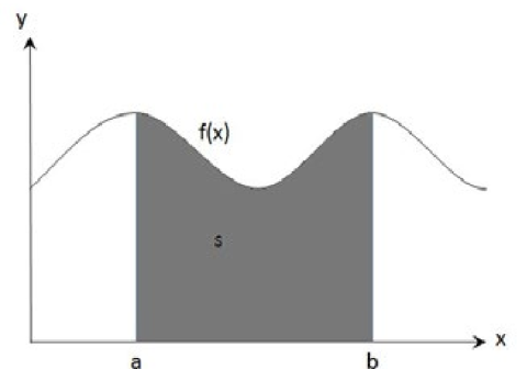
Figure 2: Differentiating velocity to obtain acceleration
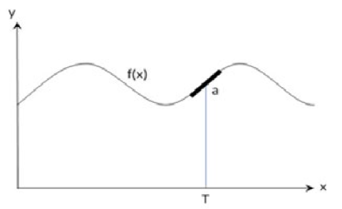
Figure 3: A simple digital signal
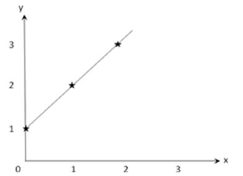
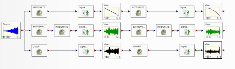
Figure 4: DATS worksheet converting from acceleration to velocity to displacement
In simple terms, these curves can be described as functions, a function being a representation of a signal. For example, in Figure 3 below, a simple signal exists.
The (x,y) coordinates for this curve are as follows in Table 1.
| X | Y |
|---|---|
| 0 | 1 |
| 1 | 2 |
| 2 | 3 |
| 3 | 4 |
| 4 | 5 |
Table 1
The pattern is clearly repeating and simple in its nature. To express the contents of Table 1 as a function would be (x, f(x)) rather than (x, y) or more commonly denoted as y = f(x). In this case, when x = 1, then y = x + 1, and so on. Therefore the function y = f(x) is actually y = x + 1, so:
f(x) = x + 1
This explains the concept of a curve or signal being expressed as a function rather than sets of coordinates. Returning to our velocity curve, if the velocity curve against time was represented as a function, it would be
v = f(t)
Where f is the function at a given time (t), the x-axis value, that produces the y-axis value v.
But as a displacement curve, it would be represented as the function,
d(t) = ∫ v.dt
Where d(t) is the displacement and dt is the change in displacement with time.
Hence, as an acceleration curve, it would be represented as the function:
a(t) = dv/dt
Where a(t) is the acceleration and dv is the change in velocity over time.
Returning from core mathematics and using DATS to visualise these conversions, we have a simple worksheet as shown in Figure 4.
This worksheet takes a vibration signal and performs integration using three different methods and then integrates again on the resulting signals. Thus, from one acceleration signal, it is possible to convert to velocity and then to displacement.
Method 1
Integration only.
Method 2
Application of a high-pass filter and then perform the integration.
Method 3
Apply the DATS Omega Arithmetic integration algorithm.
Figure 5 shows the acceleration signal measured by an accelerometer.
Figure 6 shows the velocity signal from the “integration only” method.
Figure 7 shows the velocity signal from a high-pass filter and integration method.
Figure 8 shows the velocity signal from the Omega Arithmetic integration method.
Figure 5: Acceleration signal as measured
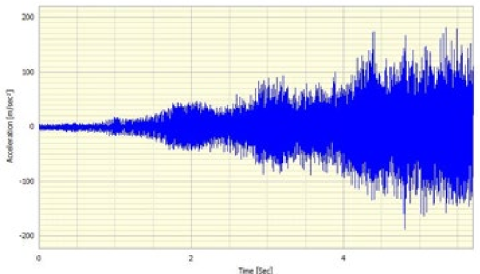
Figure 6: “Integration only” method
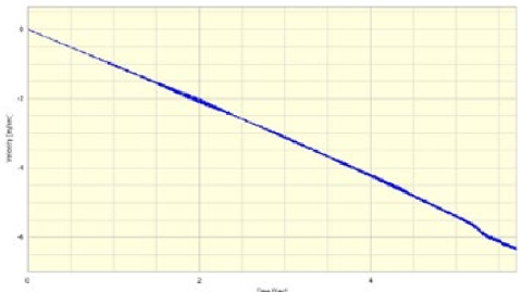
Figure 7: Velocity from high-pass filter and integration method
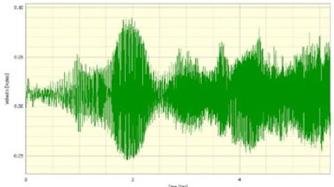
Figure 8: Velocity from Omega Arithmetic integration method
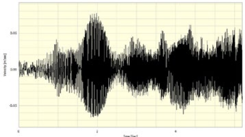
Figure 9: Displacement from integration of velocity
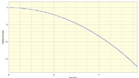
Figure 10: Displacement from high-pass filter & integration of velocity
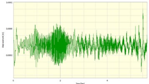
Figure 11: Displacement from Omega Arithmetic integration of velocity
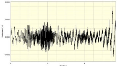
Figure 12: Velocity from methods 2 & 3
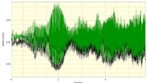
Figure 13: Displacement from methods 2 & 3
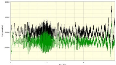
Figure 9 shows the displacement signal, created by performing the integration on a velocity signal as in Figure 6.
Figure 10 shows the displacement signal, created by performing a high-pass filter and the integration on a velocity signal as in Figure 7.
Figure 11 shows the displacement signal, created by performing the Omega Arithmetic integration on a velocity signal as in Figure 8.
These graphs show the different results from our three methods of the conversion between acceleration, velocity and displacement, pay special attention to the magnitude of the y-axis units, these reflect the conversion in question and give some guide to the accuracy of the signals.
It can be seen that, in Figure 6 and Figure 9, the integration-only method has produced results which are clearly incorrect. The displacement curve shows a movement of several metres when we know we were measuring displacements of only mm’s. The shape of the curves tells us that there is a factor or constant that is affecting the shape of the curve. The data appears to go in the same direction and is constantly increasing in magnitude. This is because of the low frequency or DC content of the signal. This causes an effect which throws out the conversion process, and the integration cannot account for this DC content. This error builds up as the signal is integrated and gives this growing or decreasing error effect. As can be seen from Figure 6, the actual valid part of the signal can just be seen but is very small; it appears to be superimposed on the growing error. It is clear from this that Method 1 is not the correct procedure.
As Figure 7 and Figure 8 show very similar signals, one might expect there to be no difference, but on closer inspection of the y-axis values, it is possible to see that the filter and integrate method has left a slight DC offset present in the signal. That is, the origin is not about zero when we know that it should be. This same pattern is repeated in Figure 9 and Figure 10. Figures 12 & 13 show the velocity and displacement from Method 2 and Method 3 superimposed.
This leaves the Omega Arithmetic method for discussion; after experimentation, it has been proven to be the only valid method.
The reason for this is that, with Omega Arithmetic, the integration is completed in the frequency domain and not in the time domain. The signal is converted to the frequency domain with an FFT, integrated or differentiated, and then, using an inverse FFT, converted back to the time domain.
In summary, if converting from Acceleration to Velocity to Displacement, the required conversion is integration; to go the other way, differentiation is used.
Simply applying calculus to a time domain signal is not an acceptable method to perform this conversion.
Filtering in the time domain to remove any DC content, for example, filtering out 5 Hz or below, then integrating does produce reasonable-looking results, but they are not correct.
The correct conversion method is Omega Arithmetic.
Have a question about this article? Email our support team
Browse all articles
Our full library of articles, tutorials and how-tos is available on the Prosig Noise and Vibration Blog.
How impact hammer testing reveals a structure's natural frequencies, damping and mode shapes, and how to get reliable results.
Why you might change the sample rate of your data, and how to do it without introducing errors such as aliasing.
What a frequency response function is, how it's measured, and how to read one to understand a structure's behaviour.
How acceleration, velocity and displacement relate to each other, with simple conversion formulas and the pitfalls to avoid.
A guide to measurement microphones: free-field, pressure and random-incidence responses, polarisation and size, and how to choose the right one.
Why window functions change the values in your spectrum, and when to apply amplitude correction or energy correction.
Have a question we haven't answered?
Get the latest DATS software updates and patches for your licensed system.
Watch Prosig systems in action, with tutorials and explainer videos on our YouTube channel.
Open and view DATS data files with our free viewer, no licence needed.
Our free 7th edition guide to sensors, measurement and analysis.
Tell us how we’re doing. Your feedback helps us improve our products and support.

From aerospace and automotive testing to condition monitoring and human vibration research, explore how Prosig's measurement solutions are applied across demanding engineering environments.
Worldwide support, local expertise
Our support team is based in the UK, with offices in the USA and a network of distributors worldwide providing local sales and support.

Our sites

Distributors